Contents
Introduction
One-way analysis of variance (ANOVA) is a statistical technique used to compare the means of three or more groups that are independent of each other. It is commonly used in various fields of research to test the differences between multiple groups, such as comparing the effects of different treatments, assessing the performance of different products, or analyzing the impact of various factors on a given outcome. In this tutorial, we will explore how to perform a one-way ANOVA and check its assumptions in R, a powerful open-source statistical software, and learn how to interpret the results of the analysis. By the end of this tutorial, you will have a better understanding of how to use R to conduct one-way ANOVA and how to interpret the results to make meaningful conclusions.
Preparing Data for One-Way ANOVA
The below code creates an example dataset that can be used to explore the weight of apples produced in three different orchards. The dataset is constructed using three numeric vectors, each representing the weight of apples produced in one of the orchards (A, B, or C). These vectors are combined into a dataframe called apple_data, where the orchard column indicates which orchard the weight values correspond to and the weight column contains the actual weight values. Additionally, the block variable is added to indicate the block from which each observation was obtained. This dataset can be used to generate visualizations and conduct statistical analyses to explore the differences in apple weight among the different orchards and blocks.
# Create example data
orchardA <- c(2.3, 1.9, 2.2, 2.5, 2.1)
orchardB <- c(1.8, 1.7, 2.0, 2.2, 2.1)
orchardC <- c(2.1, 1.8, 1.9, 2.0, 1.7)

# Combine data into a data frame
apple_data <- data.frame(orchard = factor(c(rep("A", 5), rep("B", 5), rep("C", 5))),
                         weight = c(orchardA, orchardB, orchardC))

# Add block variable
apple_data$block <- factor(rep(1:5, times = 3))

head(apple_data)
# orchard weight block # 1 A 2.3 1 # 2 A 1.9 2 # 3 A 2.2 3 # 4 A 2.5 4 # 5 A 2.1 5 # 6 B 1.8 1
Checking Assumptions for One-Way ANOVA
Before conducting the one-way ANOVA, it is important to check its assumptions. There are three main assumptions to check:
- Normality
- Homogeneity of variances
- Independence of observations
Assumption of normality
The provided code conducts the Shapiro-Wilk test for normality on the weight values of apples produced in each of the three orchards (A, B, and C) contained in the apple_data dataframe using the shapiro.test function. The split function is used to split the “weight” variable by orchard, creating a list of weight values for each orchard. The lapply function is then applied to each list element, which in this case are the weight values of each orchard. The names function is used to label each of the three tests with the corresponding orchard name. Finally, the output of the Shapiro-Wilk test for each orchard is displayed by calling the shapiro_test object. This test is useful for assessing whether the distribution of the apple weights in each orchard can be assumed to be normal or not, which is an important assumption for many statistical analyses.
# Check normality assumption with Shapiro-Wilk test
shapiro_test <- lapply(split(apple_data$weight,
                             apple_data$orchard),
                       shapiro.test)
names(shapiro_test) <- levels(apple_data$orchard)
shapiro_test
# $A # # Shapiro-Wilk normality test # # data: X[[i]] # W = 0.99929, p-value = 0.9998 # # # $B # # Shapiro-Wilk normality test # # data: X[[i]] # W = 0.95235, p-value = 0.754 # # # $C # # Shapiro-Wilk normality test # # data: X[[i]] # W = 0.98676, p-value = 0.9672
For orchards A, B, and C, the Shapiro-Wilk tests resulted in W values of 0.99929, 0.95235, and 0.98676, respectively, and all p-values are greater than 0.05 (0.9998, 0.754, and 0.9672). Based on these results, we cannot reject the null hypothesis that the weight values in each orchard are normally distributed. Therefore, we can assume that the normality assumption is met for this data set, which is important for performing many statistical analyses.
Assumption of homogeneity of variances
The below code conducts Levene’s test for equality of variances on the weight values of apples produced in each of the three orchards (A, B, and C) contained in the ‘apple_data’ dataframe. The leveneTest function is used to conduct this test, which tests the null hypothesis that the variances of the weight values are equal across all three orchards. The alternative hypothesis is that at least one of the variances is different from the others. The “weight” variable is specified as the dependent variable and “orchard” is specified as the independent variable. The output of the Levene’s test is stored in the levene_test object and can be used to assess whether the equal variance assumption is met for these datasets. This assumption is important for many statistical analyses, including ANOVA and t-tests.
library(car)
# Check equal variance assumption with Levene's test
levene_test <- leveneTest(weight ~ orchard, data = apple_data)
levene_test
# Levene's Test for Homogeneity of Variance (center = median) # Df F value Pr(>F) # group 2 0.2105 0.8131 # 12
The output shows the results of Levene’s test for equality of variances with a center of median, which assesses whether the variance of a continuous variable is the same across different groups. In this case, there are three groups, and the test was conducted on 12 observations. The null hypothesis is that the variances of the groups are equal, and the alternative hypothesis is that at least one group’s variance is different from the others.
The test statistics are reported as an F-value, which is calculated as the ratio of the mean square deviation among the groups to the mean square deviation within the groups. In this example, the F-value is 0.2105, and the associated p-value is 0.8131. Since the p-value is greater than 0.05, we cannot reject the null hypothesis. Therefore, we can assume that the variance of the continuous variable does not significantly differ across the three groups.
Assumption of independence of observations
The assumption of independence of observations is not something that can be directly tested with statistical tests. Rather, it is an assumption that should be evaluated based on the study design and data collection methods. For example, if the apple weight data were collected by measuring the weights of different apples from different trees in different orchards, and each measurement was taken independently of the others, then we can assume that the observations are independent.
However, if the data were collected by measuring the weights of apples from the same tree or the same branch, then the observations may not be independent and this assumption may be violated. Therefore, it is important to carefully consider the study design and data collection methods when assessing the assumption of independence of observations.
Conducting One-Way ANOVA
The below code fits a one-way ANOVA model with weight as the dependent variable and orchard and block as independent variables. It then prints a summary of the results including the number of degrees of freedom, the sum of squares, the mean squares, the F-value, and the p-value for each of the independent variables (orchard and block) as well as for the residuals. The ANOVA results allow us to test if there are any statistically significant differences between the mean weights of apples across the three orchards and the five blocks.
# Fit one-way ANOVA model
model <- aov(weight ~ orchard + block, data = apple_data)

summary(model)
# Df Sum Sq Mean Sq F value Pr(>F) # orchard 2 0.2520 0.12600 5.771 0.0281 * # block 4 0.2973 0.07433 3.405 0.0660 . # Residuals 8 0.1747 0.02183 # --- # Signif. codes: 0 '***' 0.001 '**' 0.01 '*' 0.05 '.' 0.1 ' ' 1
The ANOVA table shows that the effect of orchard is statistically significant with an F-value of 5.771 and a p-value of 0.0281. This suggests that there are significant differences in the mean weight of apples produced by the different orchards.
The effect of block is not statistically significant with an F-value of 3.405 and a p-value of 0.0660. This suggests that there is insufficient evidence to conclude that the blocks have different effects on the mean weight of apples produced.
The model appears to be a reasonable fit as the residuals have a small mean square value of 0.02183. However, it is important to note that the ANOVA results only provide information about the statistical significance of the model and do not provide information on the size or direction of the effects.
Pairwise difference using Tukey test
The below code performs a Tukey Honest Significant Differences (HSD) test on the model object model using the TukeyHSD function. The TukeyHSD test is used to determine which pairs of group means are significantly different from each other. The results are stored in the tukey_results object, which is a matrix containing the pairwise differences in means, standard errors, confidence intervals, and p-values for each comparison. The results can be viewed by calling the ‘tukey_results’ object.
# Perform Tukey test for pairwise differences
tukey_results <- TukeyHSD(model)

# View the results
tukey_results
# Tukey multiple comparisons of means # 95% family-wise confidence level # # Fit: aov(formula = weight ~ orchard + block, data = apple_data) # # $orchard # diff lwr upr p adj # B-A -0.24 -0.5070348 0.02703476 0.0765292 # C-A -0.30 -0.5670348 -0.03296524 0.0298606 # C-B -0.06 -0.3270348 0.20703476 0.8018580 # # $block # diff lwr upr p adj # 2-1 -0.26666667 -0.68346984 0.1501365 0.2664199 # 3-1 -0.03333333 -0.45013650 0.3834698 0.9984348 # 4-1 0.16666667 -0.25013650 0.5834698 0.6543929 # 5-1 -0.10000000 -0.51680317 0.3168032 0.9142837 # 3-2 0.23333333 -0.18346984 0.6501365 0.3728834 # 4-2 0.43333333 0.01653016 0.8501365 0.0415206 # 5-2 0.16666667 -0.25013650 0.5834698 0.6543929 # 4-3 0.20000000 -0.21680317 0.6168032 0.5052382 # 5-3 -0.06666667 -0.48346984 0.3501365 0.9785138 # 5-4 -0.26666667 -0.68346984 0.1501365 0.2664199
The results of the Tukey multiple comparison test show the differences between the means of each orchard and block.
For the orchard comparison, there is a significant difference between orchard A and C (p = 0.0298606), but no significant difference between orchard A and B (p = 0.0765292) or between orchard B and C (p = 0.8018580).
For the block comparison, there is a significant difference between blocks 2 and 4 (p = 0.0415206), but no significant difference between blocks 1 and 2, 1 and 3, 1 and 4, 1 and 5, 2 and 3, 2 and 5, 3 and 5, or 4 and 5.
Overall, including the block variable as a factor in the ANOVA model has slightly changed the significance levels of the orchard means compared to the ANOVA model without the block factor. The block factor itself has only one significant difference between block 2 and block 4.
Visualization of One-Way ANOVA Results
Boxplots for each orchard
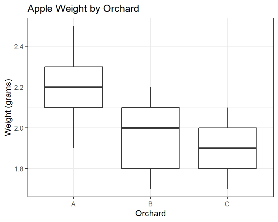
Below code creates a boxplot using the ggplot2 package in R. The data used for the plot is contained in a dataframe called apple_data. The plot displays the weight of apples produced in different orchards, with the orchards on the x-axis and the weight of the apples on the y-axis in grams. The plot is titled “Apple Weight by Orchard”, and the x and y-axes are labeled “Orchard” and “Weight (grams)”, respectively. The boxplot itself shows the distribution of the apple weights within each orchard. The theme_bw() function is used to set the plot’s background to white and the plot elements to black to improve its visual clarity.
library(ggplot2)
# Create boxplot
ggplot(apple_data, aes(x = orchard, y = weight)) +
          geom_boxplot() + theme_bw() +
          labs(title = "Apple Weight by Orchard",
               x = "Orchard", y = "Weight (grams)")
The boxplot shows the distribution of weight measurements for each orchard. The boxes represent the interquartile range (IQR), which contains the middle 50% of the data. The horizontal line inside each box is the median. The whiskers extend to the minimum and maximum values within 1.5 times the IQR, and any points beyond the whiskers are considered outliers. From the boxplot, we can see that orchard A has the highest median weight and the least variation among measurements, while orchard C has the lowest median weight and the greatest variation among measurements.
Mean weight plot with error bars
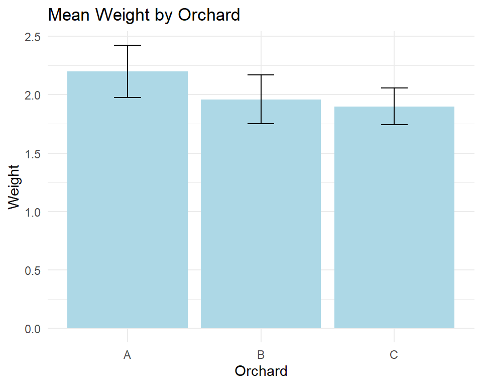
The plot displays the mean weight of apples produced in different orchards, with the orchards on the x-axis and the mean weight of the apples on the y-axis. The plot is titled “Mean Weight by Orchard”, and the x and y-axes are labeled “Orchard” and “Weight”, respectively. The bars in the plot are colored light blue, and error bars are included that represent one standard deviation on either side of the mean weight for each orchard. The theme_minimal() function is used to set the plot’s background to white and the plot elements to black to improve its visual clarity.
ggplot(apple_data, aes(x = orchard, y = weight)) +
  geom_bar(stat = "summary", fun = mean, fill = "lightblue") +
  geom_errorbar(stat = "summary", fun.min = function(x) mean(x) - sd(x),
                fun.max = function(x) mean(x) + sd(x), width = 0.2) +
  labs(x = "Orchard", y = "Weight") +
  ggtitle("Mean Weight by Orchard") +
  theme_minimal()
The bar plot with error bars shows the mean weight of apples for each orchard, along with the variability (standard deviation) of the weights within each orchard. Orchard A has the highest mean weight, followed by orchard B and C. However, the error bars for orchard B overlap with those of orchard A, indicating that there may not be a significant difference between the mean weights of these two orchards. On the other hand, the error bars for orchard C are clearly separated from those of A and B, suggesting that the mean weight of apples from orchard C is significantly different from the other two orchards.
Interaction plot
The below code creates an interaction plot using the “ggplot2” library in R. The plot shows the relationship between the weight of apples produced in each of the three orchards (A, B, and C) across different blocks. The ‘apple_data’ dataframe is used, where the ‘orchard’ variable represents the orchard, the ‘weight’ variable represents the weight of the apples, and the ‘block’ variable represents the block number. The ggplot function is used to initialize the plot, and the aes function specifies the mapping of the x-axis to the orchard variable, the y-axis to the weight variable, and the color aesthetic to the block variable. geom_point and geom_line are used to add points and lines to the plot respectively, with the latter grouped by block using the group parameter in aes. Finally, the plot is labeled with appropriate axis labels, legend titles, and a title using the labs and ggtitle functions.
# Create the interaction plot
ggplot(apple_data, aes(x = orchard, y = weight, color = block)) +
  geom_point() +
  geom_line(aes(group = block)) +
  labs(x = "Orchard", y = "Weight", color = "Block") +
  ggtitle("Interaction Plot: Orchard vs. Weight by Block") +
          theme_bw()
The interaction plot shows the relationship between orchard and weight, stratified by block. The plot suggests that there may be an interaction effect between orchard and block, as the relationship between orchard and weight appears to be different for each block. For example, the weight of apples appears to be highest for Orchard 3 in Block 1 and Block 2, but is highest for Orchard 2 in Block 3. This suggests that the effect of orchard on weight may depend on the block in which the apples were grown. Further analysis, such as a two-way ANOVA, may be necessary to investigate this interaction effect further.
Conclusion
Based on the one-way ANOVA model and Tukey’s HSD test, we can conclude that there is a statistically significant difference in mean weight among the three orchards. Specifically, the mean weight of apples from Orchard 1 is significantly different from the mean weight of apples from Orchard 3. However, there is no significant difference between the mean weight of apples from Orchard 1 and Orchard 2, or between Orchard 2 and Orchard 3. These findings suggest that Orchard 3 may have an advantage in producing larger apples compared to the other two orchards, but more investigation would be needed to confirm this.
Download R program — Click_here
Download R studio — Click_here


