Ordinal Logistic Regression: Predicting Chick Weight Categories from Diet and Time Factors

Multiple or ordinal logistic regression is a statistical technique used to model the relationship between a categorical dependent variable with three or more categories and one or more independent variables. It is an extension of binary logistic regression, which is used for binary dependent variables. This technique is commonly used in fields such as social sciences, health sciences, and business to analyze and predict outcomes based on a set of predictors.

In multiple logistic regression, the goal is to predict the probabilities of each category of the dependent variable based on the values of the independent variables. This is achieved by estimating the parameters of the model using a maximum likelihood estimation method. The parameters represent the strength and direction of the relationship between the independent variables and the dependent variable categories. The model can be used to make predictions on new data, as well as to test hypotheses about the relationships between the variables. In ordinal logistic regression, the dependent variable has an ordered structure, and the model estimates the probability of being in or below each category of the dependent variable based on the values of the independent variables.

The ordinal logistic regression model equation is given by:

$$
logit(P(Y_i \leq j)) = \beta_{0j} + \beta_1X_{i1} + \beta_2X_{i2} + \cdots + \beta_pX_{ip}
$$

where \(Y_i\) is the dependent variable representing the ordinal response for observation \(i\), \(j\) is the number of categories for the dependent variable, \(\beta_{0j}\) is the intercept for category \(j\), \(\beta_1\) to \(\beta_p\) are the coefficients for the independent variables \(X_{i1}\) to \(X_{ip}\), and \(logit(P(Y_i \leq j))\) is the log odds of the probability that \(Y_i\) is less than or equal to category \(j\).

Loading data set

The ChickWeight data set in R provides a rich source of information about the weights of chicks over time. In this dataset, each chick is weighed at regular intervals from hatching until day 21, resulting in a longitudinal dataset with multiple measurements per chick. One way to analyze this dataset is to use ordinal logistic regression, a statistical method that models the relationship between an ordinal dependent variable and one or more independent variables.

However, before we can conduct ordinal logistic regression analysis, we first need to prepare the data by creating meaningful categories for the dependent variable, which in this case is the weight of the chicks. In the following sections, we will walk through the steps of creating the weight categories and conducting ordinal logistic regression analysis in R.

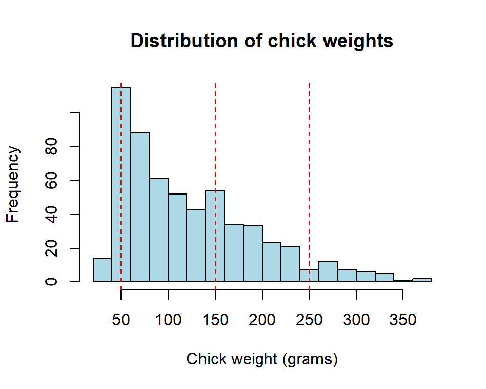
We then created a histogram of the chick weights to visualize the distribution of the data. Based on the histogram, we suggested weight ranges that correspond to different weight categories: very small, small, medium, and large.

# Load data
data("ChickWeight")

# Create histogram of chick weights
hist(ChickWeight$weight, breaks = 20, col = "lightblue",
     xlab = "Chick weight (grams)", main = "Distribution of chick weights")

# Add vertical lines to indicate suggested category boundaries
abline(v = c(50, 150, 250), lty = 2, col = "red")

We then converted the numerical weight categories in the dataset to character categories using the cut() function in R. This process of creating new variables or categories from existing data is an important step in data analysis. It allows us to better understand the data and identify patterns or trends that might not be apparent at first glance.

We used visualization techniques to identify weight ranges that correspond to meaningful categories, but there are many other ways to create new variables, such as combining existing variables or transforming variables.

# Suggest character categories
# 0-50 grams: "very small"
# 51-150 grams: "small"
# 151-250 grams: "medium"
# 251 grams and above: "large"

# Convert weight_group variable to character categories
ChickWeight$weight_group <- cut(ChickWeight$weight, 
                                breaks = c(0, 50, 150, 250, Inf), 
                                labels = c("very small", "small", "medium", "large"),
                                include.lowest = TRUE)
head(ChickWeight)

#   weight Time Chick Diet weight_group
# 1     42    0     1    1   very small
# 2     51    2     1    1        small
# 3     59    4     1    1        small
# 4     64    6     1    1        small
# 5     76    8     1    1        small
# 6     93   10     1    1        small

Now that we have the data and have created the weight_group variable with our suggested categories, we can move on to conducting an ordinal logistic regression analysis using weight_group as the outcome variable.

Model Training and Testing

Split the data into training and testing sets

When building a predictive model, it is important to evaluate its performance on data that was not used for training. This allows us to assess how well the model generalizes to new data. One way to do this is by splitting the dataset into a training set and a testing set.

In this tutorial, we will walk through the steps of converting the response variable to a factor and splitting the data into training and testing sets using the caret package in R. By doing this, we will be able to build a predictive model using the training set and evaluate its performance on the testing set.

# Converting response variable to factor
ChickWeight$weight_group <- as.factor(ChickWeight$weight_group)

# Split the data into training and testing sets
library(caret)
set.seed(125)
train_index <- createDataPartition(ChickWeight$weight_group, 
                                   p = 0.7, list = FALSE)
train <- ChickWeight[train_index, ]
test <- ChickWeight[-train_index, ]
dim(train)

# [1] 406   5

dim(test)

# [1] 172   5

Train the ordinal logistic regression model

We will demonstrate how to train an ordinal logistic regression model using the ordinal package in R. Specifically, we will use the clm() function to train an ordinal logistic regression model on a training data set, with weight_group as the ordinal response variable and Time and Diet as the predictor variables.

We will then summarize the results of the model using the summary() function.

library(ordinal)
# Train the ordinal logistic regression model on the training data
model <- clm(weight_group ~ Time + Diet, data = train)
summary(model)

# formula: weight_group ~ Time + Diet
# data:    train
# 
#  link  threshold nobs logLik  AIC    niter max.grad cond.H 
#  logit flexible  406  -204.14 422.28 8(0)  1.42e-09 2.4e+04
# 
# Coefficients:
#       Estimate Std. Error z value Pr(>|z|)    
# Time   0.63899    0.05049  12.655  < 2e-16 ***
# Diet2  1.00408    0.36113   2.780  0.00543 ** 
# Diet3  2.04702    0.37164   5.508 3.63e-08 ***
# Diet4  1.97664    0.37943   5.210 1.89e-07 ***
# ---
# Signif. codes:  0 '***' 0.001 '**' 0.01 '*' 0.05 '.' 0.1 ' ' 1
# 
# Threshold coefficients:
#                  Estimate Std. Error z value
# very small|small   2.3728     0.3302   7.185
# small|medium      10.6886     0.8620  12.399
# medium|large      14.9136     1.1077  13.464

The results indicate that ‘Time’ has a statistically significant positive effect on the likelihood of a higher weight group, with an estimated coefficient of 0.63899 (p < 0.001). This suggests that as the time progresses, the weight group is likely to increase.

Moreover, the results indicate that the effect of ‘Diet’ is also statistically significant, as indicated by the p-values of Diet2, Diet3, and Diet4, all of which are less than 0.05. These coefficients represent the difference between the baseline Diet1 and each of the other diets. The positive coefficients of Diet2, Diet3, and Diet4 indicate that these diets are associated with higher weight groups compared to Diet1. Among these diets, Diet3 has the highest coefficient, indicating the strongest positive effect on weight group.

Finally, the output also provides the estimated threshold coefficients for the cut-off points between the different levels of the ‘weight_group’ variable. These thresholds are very small|small (2.3728), small|medium (10.6886), and medium|large (14.9136). These values represent the point estimates of the cut-off values for the different levels of weight groups.

Model Interpretation

Odds Ratios

• Time: For each unit increase in Time, the estimated increase in the log odds of being in a higher weight group is 0.63899.
• Diet2: Chickens in diet group 2 have 2.7278 times higher odds of being in a lower weight group than chickens in diet group 1 (the reference group), after controlling for Time.
• Diet3: Chickens in diet group 3 have 7.7518 times higher odds of being in a lower weight group than chickens in diet group 1 (the reference group), after controlling for Time.
• Diet4: Chickens in diet group 4 have 7.2161 times higher odds of being in a lower weight group than chickens in diet group 1 (the reference group), after controlling for Time.

All predictor variables are statistically significant (p < 0.05) in predicting weight group.

The threshold coefficients are:

• very small|small: 2.3728, indicating the log odds of being in the ‘small’ group instead of the ‘very small’ group is 2.3728.
• small|medium: 10.6886, indicating the log odds of being in the ‘medium’ group instead of the ‘small’ group is 10.6886.
• medium|large: 14.9136, indicating the log odds of being in the ‘large’ group instead of the ‘medium’ group is 14.9136.

Evaluate the model on the testing data by predicting the response variable

The predict() function is used with the model object as the first argument and the testing data as the newdata argument. The type argument is set to “class” to obtain the predicted class labels rather than the predicted probabilities. The resulting pred object contains the predicted weight group categories for the testing data.

# Evaluate the model on the testing data
pred <- predict(model, newdata = test, type = "class")
head(pred$fit, n = 20)

#  [1] very small small      small      small      small      medium    
#  [7] medium     small      medium     small      medium     medium    
# [13] small      medium     very small small      small      medium    
# [19] medium     very small
# Levels: very small small medium large

The first observation in the test data is predicted to be in the “very small” weight group, the second observation is predicted to be in the “small” weight group, and so on. These predictions can be used to evaluate the performance of the model on the test data.

Create a confusion matrix to evaluate the model’s performance

The table() function in R is used to create a contingency table or confusion matrix which compares the predicted values against the actual values in the test dataset. The resulting confusion matrix can be used to evaluate the performance of the model, by comparing the number of correctly and incorrectly classified instances.

# Create a confusion matrix
cm <- table(Predicted = pred$fit, Actual = test$weight_group)
cm

#             Actual
# Predicted    very small small medium large
#   very small         22     1      0     0
#   small               3    73     10     0
#   medium              0    19     26     8
#   large               0     1      6     3

The confusion matrix compares the predicted classes with the actual classes of the testing data. The rows correspond to the predicted classes, and the columns correspond to the actual classes.

In this case:
* the model predicted 23 cases to be “very small” and they were actually “very small” in reality.
* The model predicted 3 cases to be “very small” and they were actually “small” in reality.
* The model predicted 2 cases to be “small” and they were actually “very small” in reality.
* The model predicted 78 cases to be “small” and they were actually “small” in reality, and so on.

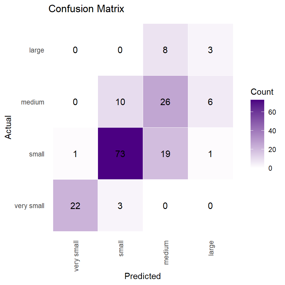
The confusion matrix shows that the model performs well in predicting the “small” category, but struggles with the “large” category.

Visualizing confusion matrix

We can create visualization of a confusion matrix using the ggplot2 library. The reshape2 library is used to convert the matrix object into a data frame. The ggplot() function is then used to create the visualization, with geom_tile() and scale_fill_gradient() functions used to display the data as a heatmap.

The geom_text() function is used to add counts to each tile of the heatmap, and theme_minimal() is used to simplify the appearance of the plot. Finally, the labs() function is used to add labels and a title to the plot. The resulting plot is an informative and visually appealing visualization of the confusion matrix.

library(reshape2)
library(ggplot2)
# convert confusion matrix to a data frame
confusion_matrix_df <- melt(cm)

# plot confusion matrix using ggplot2
ggplot(confusion_matrix_df, aes(x = Predicted, y = Actual, fill = value)) +
  geom_tile(color = "white") +
  scale_fill_gradient(low = "white", high = "#4b0082") +
          geom_text(aes(label = value), color = "black", size = 4) +
  theme_minimal() +
  theme(
        panel.grid.major = element_blank(),
        panel.grid.minor = element_blank(),
        axis.text.x = element_text(angle = 90, vjust = 0.5, hjust=1)) +
  labs(title = "Confusion Matrix", x = "Predicted", y = "Actual",  
       fill = "Count")

Calculate the accuracy of the model

Accuracy of the model is calculated by dividing the sum of diagonal elements of the confusion matrix by the total number of observations. The diagonal elements represent the number of correctly classified instances, while the off-diagonal elements represent the number of incorrectly classified instances.

Dividing the sum of diagonal elements by the total number of observations gives the proportion of correctly classified instances. This accuracy metric can be used to evaluate the performance of the model.

# Calculate accuracy
accuracy <- sum(diag(cm)) / sum(cm)
paste(round(accuracy, digits = 3)*100, "%") 

# [1] "72.1 %"

The accuracy of the model on the testing data is 72.1%. This means that the model correctly predicted the weight group for 72.1% of the observations in the testing dataset.

Conclusion

In this blog post, we trained an ordinal logistic regression model on the ChickWeight dataset to predict the weight group category based on the diet and time factors. We split the dataset into training and testing sets, trained the model, and evaluated its performance using a confusion matrix. The results indicate that the model has a good performance in predicting the weight group categories. Overall, this technique is a valuable tool in modeling and predicting categorical outcomes based on a set of predictors.

---

Download R program — Click_here

Download R studio — Click_here