Linear regression is a powerful tool for understanding the relationship between two variables. In this blog, we will explore how to use simple linear regression in R and gain insights into our data. We’ll cover following topics:
- What Is Simple Linear Regression?
- Loading iris dataset
- Fitting a simple linear regression model with lm() Function
- Interpreting Results of the Model Fit
- Visualizing the Relationship Between Variables
Contents
What Is Simple Linear Regression?
Simple linear regression is used to analyze relationships between two continuous variables – an independent variable (x) and dependent variable (y). It assumes that there exists some kind of linear relationship between these two variables, which can be expressed by a straight line on a graph. The goal of simple linear regression is to find out what parameters best describe this line so that it fits our data points as closely as possible. This process involves estimating coefficients for each variable and then using them to calculate predicted values from new observations.
The output of a simple linear regression model includes an equation of the form:
$$\gamma = \beta_0 + \beta_1X + \epsilon$$
where \(\beta_0\) is the intercept, \(\beta_1\) is the slope coefficient, and \(\epsilon\) is the error term. The slope coefficient (\(\beta_1\)) represents the change in the response variable (\(\gamma\)) for a one-unit increase in the predictor variable (\(X\)), while holding all other variables constant. The intercept (\(\beta_0\)) represents the expected value of the response variable (\(\gamma\)) when the predictor variable (\(X\)) is equal to zero.
Loading iris data
In R, you can load the iris dataset by simply calling the data() function and passing in the name of the dataset as a parameter. This will load the iris dataset into R and make it available for use in your R session. Once the dataset is loaded, you can view the first few rows of the dataset using the head() function. This will print out the first 6 rows of the iris dataset, which includes the variables “Sepal.Length”, “Sepal.Width”, “Petal.Length”, “Petal.Width”, and “Species”.
data("iris")
head(iris)
# Sepal.Length Sepal.Width Petal.Length Petal.Width Species # 1 5.1 3.5 1.4 0.2 setosa # 2 4.9 3.0 1.4 0.2 setosa # 3 4.7 3.2 1.3 0.2 setosa # 4 4.6 3.1 1.5 0.2 setosa # 5 5.0 3.6 1.4 0.2 setosa # 6 5.4 3.9 1.7 0.4 setosa
Fitting simple linear regressoin model
For example, let’s say we want to fit a simple linear model where \(y=a+bx\), where \(a\) stands for intercept value while \(b\) represents slope coefficient; both of which need estimation based on given input data points \(x\) & \(y\).
In our example we shall see the relationship between Sepal.Length and Petal.Length specifying x and y variables in the regression model, respectively. To fit a linear regression model to predict the variable Petal.Length based on Sepal.Length, we can use lm() from stats package to create and fit our linear regression model with Sepal.Length as an explanatory variable and Petal.Length as a response variable.
This function takes three arguments: formula = y ~ x1 + x2 + … , data = data object, family = gaussian. The formula argument specifies which variables will be included in our model while data tells us which dataset should be used when fitting our model. Finally family defines type of distribution being modeled here – Gaussian being most common choice but other options exist too such as binomial or poison depending upon situation at hand.
After running this command our fitted model object will be stored inside fit object ready for interpretation!
fit <- lm(formula = Petal.Length ~ Sepal.Length,
          data = iris,
          family = Gaussian)
Interpretting results of the model fit
The output of this code will be the linear regression model, which includes the intercept and slope coefficients, as well as other information such as the residuals and R-squared value.
To view a summary of the model, we can use the summary() function:
summary(fit)# # Call: # lm(formula = Petal.Length ~ Sepal.Length, data = iris, family = Gaussian) # # Residuals: # Min 1Q Median 3Q Max # -2.47747 -0.59072 -0.00668 0.60484 2.49512 # # Coefficients: # Estimate Std. Error t value Pr(>|t|) # (Intercept) -7.10144 0.50666 -14.02 <2e-16 *** # Sepal.Length 1.85843 0.08586 21.65 <2e-16 *** # --- # Signif. codes: 0 '***' 0.001 '**' 0.01 '*' 0.05 '.' 0.1 ' ' 1 # # Residual standard error: 0.8678 on 148 degrees of freedom # Multiple R-squared: 0.76, Adjusted R-squared: 0.7583 # F-statistic: 468.6 on 1 and 148 DF, p-value: < 2.2e-16
The output of this code will include various statistics about the model, including the coefficients, standard errors, t-values, and p-values. The Sepal.length is strongly correlated with Petal.length as indicated by the lower p value (p < 0.001) and this association is positive indicating with increase in Sepal.length there is also increase in Petal.length.
The intercept can be interpreted as the expected value of the response variable (Y) when the predictor variable (X) is equal to zero. However, this interpretation may not be meaningful in all cases, depending on the context of the analysis.
The slope coefficient represents the change in the response variable (Y) for a one-unit increase in the predictor variable (X), while holding all other variables constant. In this example, the slope coefficient is 1.86, then we would expect the Petal length (Y) to increase by 1.86 units for every one-unit increase in the Sepal length (X).
R-squared, also known as the coefficient of determination, is a statistical measure that indicates the proportion of the variance in the dependent variable that is explained by the independent variable(s) in a regression model. In other words, R-squared measures how well the independent variable(s) can predict the variation in the dependent variable.
R-squared is a value between 0 and 1. A value of 0 indicates that the independent variable(s) cannot explain any of the variation in the dependent variable, while a value of 1 indicates that the independent variable(s) can perfectly explain all of the variation in the dependent variable.
In our example we can roughly say around 76% of the variability in Petal length is explained by the Sepal length. This also indicates that a large proportion of the variability in the Petal length was explained by the Sepal length in iris data.
Visualizing the relationship between variables
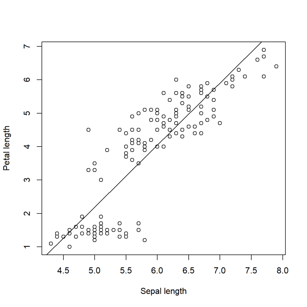
Once we’re done interpreting results from previous steps it’s always helpful visualize actual relationship between x & y variables via plotting scatter plot together with corresponding fitted line representing equation derived.
We can plot the data and the linear regression line using the plot() and abline() functions.
plot(
          iris$Sepal.Length, iris$Petal.Length,
          xlab = "Sepal length",
          ylab = "Petal length"
)
abline(fit)
This will create a scatter plot of the data with the linear regression line overlaid on top.
Note that in this example, we assumed that the data is already in a data frame format. If the data is in a different format, such as a matrix or a vector, we may need to convert it to a data frame using the data.frame() function before fitting the linear regression model.
Download R program — Click_here
Download R studio — Click_here


