In this blog post, we will do exploration of the Nile River’s annual streamflow data using time series analysis. The data, which spans from 1871 to 1970, offers a rich context for understanding the river’s flow patterns over time. We will employ ARIMA models, a popular choice for time series forecasting, to analyze this data. The process involves identifying the optimal parameters for our model, fitting the model to the data, and then generating forecasts. By comparing different ARIMA models, we aim to select the one that best fits our data and provides the most accurate forecasts.
Let’s start!
Contents
Introduction
We will use the famous Nile River’s annual streamflow data, conveniently stored in a time series data set named Nile. This dataset goes beyond just numbers; it also includes metadata, providing valuable context. When you call print(Nile), you’ll see details like Start = 1871, indicating the first year of data collection, and End = 1970, marking the final year covered in this specific dataset.
data("Nile")
print(Nile)
## Time Series: ## Start = 1871 ## End = 1970 ## Frequency = 1 ## [1] 1120 1160 963 1210 1160 1160 813 1230 1370 1140 995 935 1110 994 1020 ## [16] 960 1180 799 958 1140 1100 1210 1150 1250 1260 1220 1030 1100 774 840 ## [31] 874 694 940 833 701 916 692 1020 1050 969 831 726 456 824 702 ## [46] 1120 1100 832 764 821 768 845 864 862 698 845 744 796 1040 759 ## [61] 781 865 845 944 984 897 822 1010 771 676 649 846 812 742 801 ## [76] 1040 860 874 848 890 744 749 838 1050 918 986 797 923 975 815 ## [91] 1020 906 901 1170 912 746 919 718 714 740
To make sure the Nile is a time series data you can use is.ts() and class() function to verify this.
is.ts(Nile)## [1] TRUE
class(Nile)## [1] "ts"
The plot() function visualizes the historical flow patterns of data. We can observe variations in flow throughout the years, potentially indicating trends or long-term changes.
plot(Nile)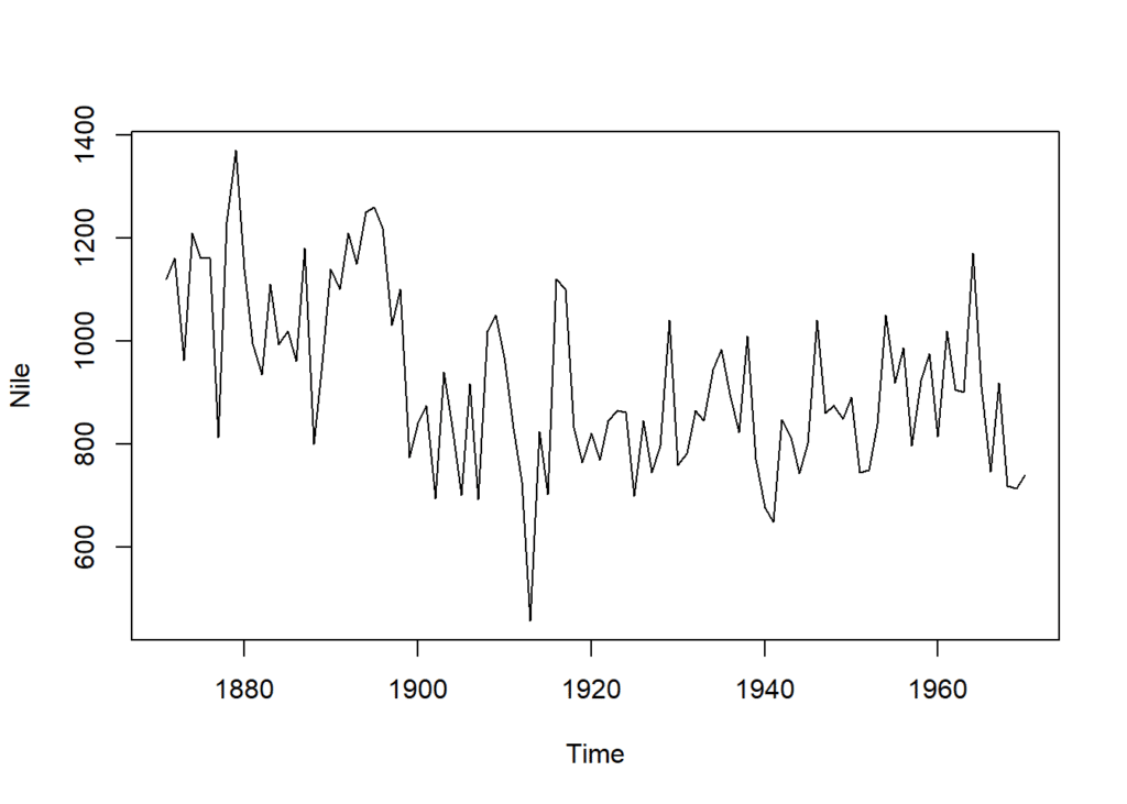
Model Identification
We shall use the two most commonly used functions (acf and pacf) to analyze the time series properties of this data.
par(mfrow = c(1,2))
acf(Nile)
pacf(Nile)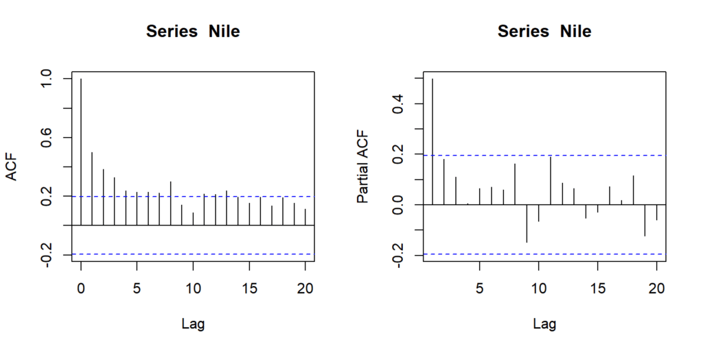
Based on the partial autocorrelation (ACF) plot in the image, it appears that an ARIMA order of (1, 1, 0) might be appropriate. This is because the ACF plot shows a single spike at lag 1, and then dies off afterwards. This suggests that there is an autoregressive term of order 1 (AR(1)) in the model, but no higher order terms are needed. Further we can also see that the autocorrelation values also do not come to zero reasonably quickly, indicates no-stationarity and the series need to be differenced. The autocorrelation (ACF) plot also shows some spikes that cut off after a few lags, but they are not as clear-cut as the PACF plot. This further suggests that a moving average term (MA) is not required in the model (MA(0)).
There is no evidence in the plots to suggest that a seasonal component should be included in the model. The PACF and ACF plots do not exhibit any periodic patterns, which would be indicative of a seasonal component.
Based on these facts we will select ARIMA model of order (1, 1, 0).
Let’s use the auto.arima() function to identify the optimal order for ARIMA model for this time series data. This function will automatically search for the best combination of parameters (p, d, q) based on statistical criteria.
library(forecast)
auto.arima(Nile)
## Series: Nile ## ARIMA(1,1,1) ## ## Coefficients: ## ar1 ma1 ## 0.2544 -0.8741 ## s.e. 0.1194 0.0605 ## ## sigma^2 = 20177: log likelihood = -630.63 ## AIC=1267.25 AICc=1267.51 BIC=1275.04
Fitting ARIMA models
While auto.ARIMA suggests ARIMA(1,1,1), it’s wise to compare it to ARIMA(1,1,0) (from the ACF plot) and ARIMA(1,0,0) (no differencing). This will ensure to select the best possible model by comparing their characteristics.
# Fit an AR model to Nile
Auto_fit <- auto.arima(Nile)
AR_fit <- arima(Nile, order = c(1, 0, 0))
ARd_fit <- arima(Nile, order = c(1, 1, 0))
Comparing ARIMA models
We can use statistical tests like AIC (Akaike Information Criterion) or BIC (Bayesian Information Criterion) to see which model achieves a better fit for this data.
# Define the model fits
fits <- list(Auto_fit, AR_fit, ARd_fit)
fit_names <- c("Auto_fit", "AR_fit", "ARd_fit")

# Initialize an empty data frame
results_df <- data.frame(AIC = numeric(length(fits)),
                         BIC = numeric(length(fits)),
                         row.names = fit_names)

# Calculate AIC and BIC for each model and store in the data frame
for (i in seq_along(fits)) {
  results_df[i, "AIC"] <- AIC(fits[[i]])
  results_df[i, "BIC"] <- BIC(fits[[i]])
}

# Print the results data frame
print(results_df)
## AIC BIC ## Auto_fit 1267.255 1275.040 ## AR_fit 1285.904 1293.720 ## ARd_fit 1281.480 1286.671
Both AIC (1267.255) and BIC (1275.04) for Auto_fit are lower than the corresponding values for AR_fit and ARd_fit. Generally, lower AIC and BIC indicate a better fit for the data. While the difference in AIC between Auto_fit and ARd_fit is relatively small (around 14), it still suggests a slight preference for Auto_fit. BIC also favors Auto_fit with a clearer margin.
Generating Forecasts
Given that the ARIMA(1,1,1) model demonstrated a better fit compared to the other two models, we can proceed with generating 10-step forecasts using this model. It’s important to remember that these forecasts are based on the assumption that the underlying patterns in the data will continue to hold for the forecasted period.
While the ARIMA(1,1,1) model will be our primary forecast due to its superior fit, it can also be informative to generate forecasts for the other two models. This comparison can help us visualize the potential range of future values and assess the confidence level in our primary forecast.
# Use predict to make 1-step through 10-step forecasts
Auto_pred <- predict(Auto_fit, n.ahead = 10)
AR_pred <- predict(AR_fit, n.ahead = 10)
ARd_pred <- predict(ARd_fit, n.ahead = 10)
Comparing ARIMA Model Forecasts
This code block generates three visualizations comparing the forecasted Nile River streamflow using different ARIMA models. The par(mfrow = c(3,1)) line sets up a grid layout with three rows and one column to display the plots efficiently.
The ts.plot() line displays the actual Nile River streamflow data (Nile) along with a time axis limited to the years 1871 to 1980 (xlim). The points() function plots the predicted streamflow values (stored in Auto_pred$pred) as a red line.
par(mfrow = c(3,1))
# Predictions of Auto model ARIMA(1, 1, 1)
ts.plot(Nile, xlim = c(1871, 1980),
        ylab = "Nile River Flow",
        main = "Predictions of Auto_fit model ARIMA(1, 1, 1)")
points(Auto_pred$pred, type = "l", col = "red")
points(Auto_pred$pred - Auto_pred$se, type = "l", col = "red", lty = 2)
points(Auto_pred$pred + Auto_pred$se, type = "l", col = "red", lty = 2)

# Predictions of AR model ARIMA(1, 0, 0)
ts.plot(Nile, xlim = c(1871, 1980),
        ylab = "Nile River Flow",
        main = "Predictions of AR_fit model ARIMA(1, 0, 0)")
points(AR_pred$pred, type = "l", col = "red")
points(AR_pred$pred - AR_pred$se, type = "l", col = "red", lty = 2)
points(AR_pred$pred + AR_pred$se, type = "l", col = "red", lty = 2)

# Predictions of ARd model ARIMA(1, 1, 0)
ts.plot(Nile, xlim = c(1871, 1980), ylab = "Nile River Flow",
        main = "Predictions of ARd_fit model ARIMA(1, 1, 0)")
points(ARd_pred$pred, type = "l", col = "red")
points(ARd_pred$pred - ARd_pred$se, type = "l", col = "red", lty = 2)
points(ARd_pred$pred + ARd_pred$se, type = "l", col = "red", lty = 2)
Here are some observations based on the above predictions:
- Auto_fit model provided relatively small prediction ranges and standard errors compared to the other two models, indicating potentially more precise predictions.
- AR_fit model has larger prediction ranges but still reasonable standard errors, suggesting moderate precision.
- ARd_fit model has the smallest prediction range but also the largest standard errors, indicating potentially less reliable predictions due to higher uncertainty.
We can enhance the visualization of predictions from various models using the ggplot function, enabling more effective comparisons.
# Initialize an empty list to store the data frames
pred_dfs <- list()

# Loop through the models and make forecasts
models <- list(Auto_fit, AR_fit, ARd_fit)
model_names <- c("Auto_pred", "AR_pred", "ARd_pred")
for (i in seq_along(models)) {
  pred <- predict(models[[i]], n.ahead = 10)
  pred_df <- data.frame(
    x = c(time(pred$pred)),
    pred = c(pred$pred),
    se = c(pred$se)
  )
  pred_dfs[[i]] <- cbind(pred_df, model = model_names[i])
}

# Combine the data frames into one
combined_df <- do.call(rbind, pred_dfs)


# Load required libraries
library(ggplot2)

# Plotting
ggplot(
  combined_df, aes(x = x, y = pred, color = model)
) +
  geom_line(linewidth = 1) +
  geom_ribbon(
    aes(ymin = pred - se, ymax = pred + se, fill = model),
    alpha = 0.3, lty = 2
  ) +
  labs(x = "Year",
       y = expression("Predicted flow of River Nile (m"^3*")"),
       title = "Prediction with Standard Error") +
  theme_minimal() +
  scale_x_continuous(breaks = seq(1971, 1980, by = 2))  +
  facet_wrap(facets = ~model) +
  theme(legend.position = "none")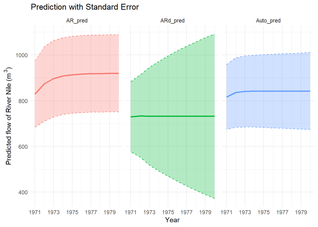
Conclusion
This analysis of the Nile River’s annual streamflow data demonstrated the utility of ARIMA models for time series forecasting. The ARIMA(1,1,1) model was identified as the best fit for the data, outperforming the ARIMA(1,0,0) and ARIMA(1,1,0) models according to AIC and BIC criteria. The forecasts generated by the ARIMA(1,1,1) model were more precise, as indicated by smaller prediction ranges and standard errors. However, it’s important to remember that these forecasts are based on the assumption that the underlying patterns in the data will continue to hold for the forecasted period. This analysis underscores the importance of model selection in time series forecasting and the value of comparing different models to ensure the best possible predictions.
For more details and informative videos you can also subscribe to our YouTube Channel AGRON Info Tech.
Download R program and R studio —
Click_here

